Next: Exact predictive density
Up: Regression
Previous: Regression
Contents
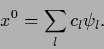
An important special case of density estimation
leading to quadratic data terms
is regression for independent training data
with Gaussian likelihoods
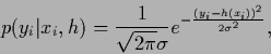 |
(245) |
with fixed, but possibly  -dependent, variance
  .
In that case
.
In that case  =
=
 is specified by
  =
=  and
the logarithmic term
and
the logarithmic term
 becomes quadratic in the regression function
  ,
i.e., of the form (225).
In an interpretation as empirical risk minimization
quadratic error terms corresponds to the choice of
a squared error loss function
,
i.e., of the form (225).
In an interpretation as empirical risk minimization
quadratic error terms corresponds to the choice of
a squared error loss function  =
=  for action
 .
Similarly, the
technical analogon of Bayesian priors
are additional (regularizing) cost terms.
.
Similarly, the
technical analogon of Bayesian priors
are additional (regularizing) cost terms.
We have remarked in Section 2.3
that for continuous  measurement
of
measurement
of  has to be understood as
measurement of a
has to be understood as
measurement of a
 =
=
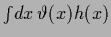 for sharply peaked
  .
We assume here that the discretization
of
.
We assume here that the discretization
of  used in numerical calculations takes care of that averaging.
Divergent quantities like
used in numerical calculations takes care of that averaging.
Divergent quantities like  -functionals,
used here for convenience, will then not be present.
-functionals,
used here for convenience, will then not be present.
We now combine Gaussian data terms and a Gaussian (specific) prior
with prior operator
 and define for training data ,
  the operator
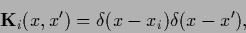 |
(246) |
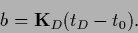
and training data templates  .
We also allow a general prior template
.
We also allow a general prior template  but remark that it is often chosen identically zero.
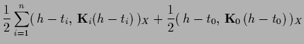
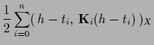
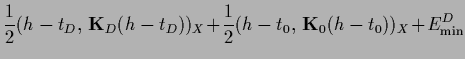
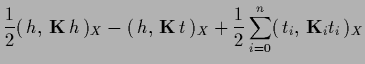
According to (230) the resulting functional can be written
in the following forms, useful for different purposes,
but remark that it is often chosen identically zero.
According to (230) the resulting functional can be written
in the following forms, useful for different purposes,
 |
 |
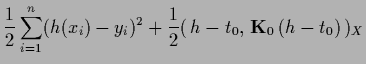 |
(247) |
| |
|
 |
(248) |
| |
|
 |
(249) |
| |
|
 |
(250) |
| |
|
 |
(251) |
| |
|
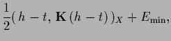 |
(252) |
with
 |
(253) |
 |
(254) |
and
-independent minimal errors,
being proportional to the ``generalized variances''
 =
=
 and
and
 =
=
 .
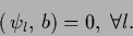
The scalar product
.
The scalar product
 stands for -integration only,
for the sake of simplicity however, we will skip the subscript
stands for -integration only,
for the sake of simplicity however, we will skip the subscript  in the following.
The data operator
in the following.
The data operator 
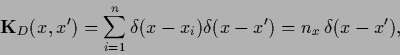 |
(257) |
contains for discrete on its diagonal
the number of measurements at ,
 |
(258) |
which is zero for not in the training data.
As already mentioned for continuous a integration
around a neighborhood of is required.
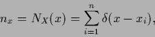
 is a short hand notation for
the inverse within the space of training data
is a short hand notation for
the inverse within the space of training data
 |
(259) |
 denoting
the projector into the space of training data
denoting
the projector into the space of training data
 |
(260) |
Notice that the sum is not over all  training points
but only over the
training points
but only over the  different .
(Again for continuous an integration around is required
to ensure
different .
(Again for continuous an integration around is required
to ensure  = ).
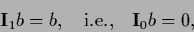
Hence, the data template
= ).
Hence, the data template
 becomes the mean of
  -values measured at
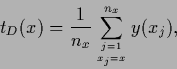 |
(261) |
and  =
=  for
for  = .
Normalization of is not influenced by a change in
so the Lagrange multiplier terms have been skipped.
= .
Normalization of is not influenced by a change in
so the Lagrange multiplier terms have been skipped.
The stationarity equation is most easily obtained from (252),
 |
(262) |
It is linear and has on a space where
 exists
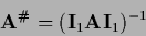
the unique solution
exists
the unique solution
 |
(263) |
We remark that  can be invertible
(and usually is so the learning problem is well defined)
even if
can be invertible
(and usually is so the learning problem is well defined)
even if  is not invertible.
The inverse
, necessary to calculate
is not invertible.
The inverse
, necessary to calculate  ,
is training data dependent
and represents the covariance operator/matrix
of a Gaussian posterior process.
In many practical cases, however, the prior covariance
,
is training data dependent
and represents the covariance operator/matrix
of a Gaussian posterior process.
In many practical cases, however, the prior covariance
 (or in case of a null space a pseudo inverse of )
is directly given or can be calculated.
Then an inversion of a finite dimensional matrix
in data space is sufficient to find the minimum of the energy
(or in case of a null space a pseudo inverse of )
is directly given or can be calculated.
Then an inversion of a finite dimensional matrix
in data space is sufficient to find the minimum of the energy  [228,76].
Invertible  :
Let us first study the case of an invertible
and consider the stationarity equation
as obtained from (248) or (250)
:
Let us first study the case of an invertible
and consider the stationarity equation
as obtained from (248) or (250)
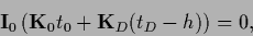
For existing
 |
(266) |
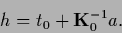
one can introduce
 |
(267) |
to obtain
 |
(268) |
Inserting Eq. (268) into Eq. (267) one finds
an equation for 
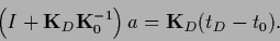 |
(269) |
Multiplying Eq. (269)
from the left by the projector
defined in (260)
and using
 |
(270) |
one obtains an equation in data space
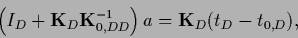 |
(271) |
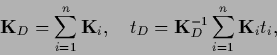
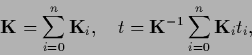
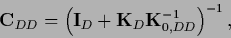
where
 |
(272) |
Thus,
 |
(273) |
where
 |
(274) |
and
 |
(275) |
In components Eq. (273) reads,
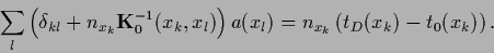 |
(276) |
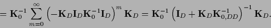
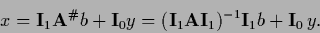
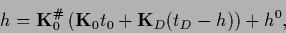
Having calculated the solution
is given by Eq. (268)
 |
(277) |
Eq. (277)
can also be obtained directly from
Eq. (263) and the definitions (254),
without introducing the auxiliary variable ,
using the decomposition
 =
=
 +
+
 and
and
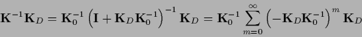 |
(278) |
 |
(279) |
 is also known as equivalent kernel
due to its relation to kernel smoothing techniques
[210,94,90,76].
is also known as equivalent kernel
due to its relation to kernel smoothing techniques
[210,94,90,76].
Interestingly,
Eq. (268) still holds
for non-quadratic data terms
of the form  with any differentiable function
fulfilling
with any differentiable function
fulfilling
 =
=  ,
where
,
where  =
=  is the restriction of to data space.
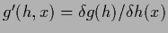
Hence, also
the function of functional derivatives
with respect to
is the restriction of to data space.
Hence, also
the function of functional derivatives
with respect to  is restricted to data space, i.e.,
 =
=
 with
with  =
=
 and
and
 .
For example,
=
.
For example,
=
 with a differentiable function.
The finite dimensional vector
is then found by solving a nonlinear equation instead of a linear one
[73,75].
with a differentiable function.
The finite dimensional vector
is then found by solving a nonlinear equation instead of a linear one
[73,75].
Furthermore, one can study vector fields, i.e., the case where,
besides possibly ,
also , and thus , is a vector for given .
(Considering the variable indicating the vector components of
as part of the -variable,
this is a situation where a fixed number of one-dimensional ,
corresponding to a subspace of with fixed dimension,
is always measured simultaneously.)
In that case the diagonal  of Eq. (246)
can be replaced by a version with non-zero off-diagonal elements
of Eq. (246)
can be replaced by a version with non-zero off-diagonal elements
 between the vector components
  of .
This corresponds
to a multi-dimensional Gaussian data generating probability
of .
This corresponds
to a multi-dimensional Gaussian data generating probability
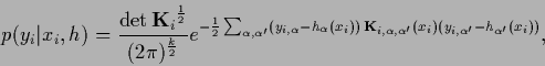 |
(280) |
for  -dimensional vector with components
  .
.
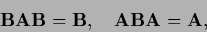
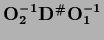
Non-invertible :
For non-invertible
one can solve for
using the Moore-Penrose inverse
 .
Let us first recall some basic facts
[58,164,186,187,126,15,120].
A pseudo inverse
.
Let us first recall some basic facts
[58,164,186,187,126,15,120].
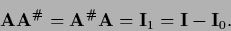
A pseudo inverse  of (a possibly non-square)
  is defined by the conditions
 |
(281) |
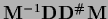
and becomes for real
the unique Moore-Penrose inverse  if
if
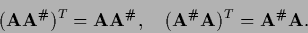 |
(282) |
A linear equation
 |
(283) |
is solvable if
 |
(284) |
In that case the solution is
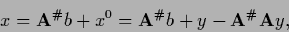 |
(285) |
where
 is solution of the homogeneous equation
 and vector is arbitrary.
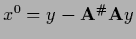
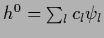
Hence,
and vector is arbitrary.
Hence,  can be expanded in an orthonormalized basis
  of the null space of
 |
(286) |
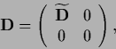
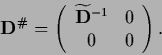
For a diagonal
 |
(287) |
where
 is invertible,
the Moore-Penrose inverse is
is invertible,
the Moore-Penrose inverse is
 |
(288) |
For a square matrix  the product
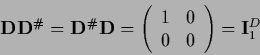 |
(289) |
becomes the projector on the space where
is invertible.
Similarly,
 =
=
 is the projector on the null space of .
For a general (possible non-square)
there always exist orthogonal  and
and  so it can be written in orthogonal normal form
=
so it can be written in orthogonal normal form
=
 ,
where is of the form of Eq. (287)
[120].
The corresponding Moore-Penrose inverse is
=
,
where is of the form of Eq. (287)
[120].
The corresponding Moore-Penrose inverse is
=
 .
.
Similarly, for an which can be diagonalized, i.e.,
for a square matrix =
 with diagonal ,
the Moore-Penrose inverse is
=
with diagonal ,
the Moore-Penrose inverse is
=
 .
From Eq. (289) it follows then that
.
From Eq. (289) it follows then that
 |
(290) |
where
 =
=
 =
=
 projects on the space where is invertible
and
projects on the space where is invertible
and
 =
=
 =
=
 is the projector into the null space of .
Then from the definition (281)
it follows
is the projector into the null space of .
Then from the definition (281)
it follows
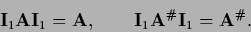 |
(291) |
Sometimes it is convenient to write
in that case
 |
(292) |
where the inversion is understood to be performed in the subspace
where is invertible.
Expressed by projectors the solvability condition Eq. (284)
becomes
 |
(293) |
or in terms of a basis of the null space
 |
(294) |
This means that the inhomogeneity  must have no components
within the null space of .
Furthermore we can then write
must have no components
within the null space of .
Furthermore we can then write
 |
(295) |
showing that an can be obtained by projecting an arbitrary
on the null space of .
Collecting the results for an
which can be diagonalized,
Eq. (285)
can be expressed in terms of projection operators as follows:
 |
(296) |
Thus a solution is obtained by inverting
in the subspace where it is invertible
and adding an arbitrary component of the null space.
Now we apply this to Eq. (265)
where is
diagonalizable because being positive semi-definite.
(In this case  is an orthogonal matrix
and the entries of
is an orthogonal matrix
and the entries of  are real and larger or equal to zero.)
Hence, one obtains under the condition
are real and larger or equal to zero.)
Hence, one obtains under the condition
 |
(297) |
for Eq. (285)
 |
(298) |
where
 =
so that
=
so that
 can be expanded in an orthonormalized basis
of the null space of , assumed here
to be of finite dimension.
To find an equation in data space
define the vector
can be expanded in an orthonormalized basis
of the null space of , assumed here
to be of finite dimension.
To find an equation in data space
define the vector
|
(299) |
to get from Eqs.(297) and (298)
These equations have to be solved for and the coefficients  .
Inserting Eq. (301) into the
definition (299) gives
.
Inserting Eq. (301) into the
definition (299) gives
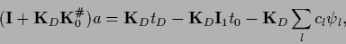 |
(302) |
using
 =
according to Eq. (290).
Using =
=
according to Eq. (290).
Using =  [where ,
the projector on the space of training data,
is defined in (260)]
the solvability condition (297) becomes
[where ,
the projector on the space of training data,
is defined in (260)]
the solvability condition (297) becomes
 |
(303) |
the sum going over different only.
Eq. (302) for and
reads in data space,
similar to Eq. (271),
 |
(304) |
where
 =
=
 has been assumed invertible
and
has been assumed invertible
and  is given by the right hand side of Eq. (302).
Inserting into Eq. (301)
the solution finally can be written
is given by the right hand side of Eq. (302).
Inserting into Eq. (301)
the solution finally can be written
 |
(305) |
Again, general non-quadratic data terms can be allowed.
In that case
 =
=
 =
=
 and Eq. (299)
becomes the nonlinear equation
and Eq. (299)
becomes the nonlinear equation
 |
(306) |
The solution(s) of that equation have then to be inserted
in Eq. (301).
Next: Exact predictive density
Up: Regression
Previous: Regression
Contents
Joerg_Lemm
2001-01-21