Prior mixtures for density estimation

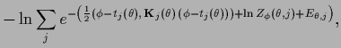
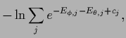
The mixture approach (535) leads in general to non-convex error functionals. For Gaussian components Eq. (535) results in an error functional

$$E_{\theta,\phi} = -(\ln P(\phi),\,N) + (P(\phi),\, \Lambda_X )$$

$$- \ln \sum_j e^{-\left( \frac{1}{2} \left(\phi-t_j(\theta),\,{{\b... ...heta)\,(\phi-t_j(\theta))\right) +\ln Z_\phi (\theta,j)+E_{\theta,j} \right)} ,$$ (536)

$$= -\ln \sum_j e^{-E_{\phi,j}-E_{\theta,j}+c_j},$$ (537)

where

$$E_{\phi,j} = -(\ln P(\phi),\,N) + (P(\phi),\, \Lambda_X ) +\... ...-t_j(\theta),\,{{\bf K}}_j (\theta)\,(\phi-t_j(\theta))\Big) ,$$ (538)

and

$$c_j = -\ln Z_\phi (\theta,j) .$$ (539)

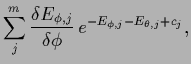
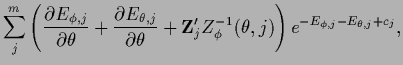
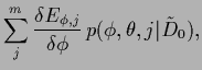
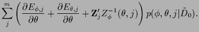
The stationarity equations for $\phi$ and $\theta$

$$0 = \sum_j^m \frac{\delta E_{\phi,j}}{\delta \phi}\, e^{-E_{\phi,j}-E_{\theta,j}+c_j},$$ (540)

$$0 = \sum_j^m \left( \frac{\partial E_{\phi,j}}{\partial \theta} +\fra... ...bf Z}_j^\prime Z_\phi^{-1}(\theta,j) \right) e^{-E_{\phi,j}-E_{\theta,j}+c_j} ,$$ (541)

can also be written

$$0 = \sum_j^m \frac{\delta E_{\phi,j}}{\delta \phi}\, p(\phi,\theta,j\vert\tilde D_0),$$ (542)

$$0 = \sum_j^m \left( \frac{\partial E_{\phi,j}}{\partial \theta} +\fra... ...\bf Z}_j^\prime Z_\phi^{-1}(\theta,j) \right) p(\phi,\theta,j\vert\tilde D_0) .$$ (543)

Analogous equations are obtained for parameterized $\phi(\xi)$.