[@twocolumnfalse
J. C. Lemm, J. Uhlig, and A. Weiguny
September 12, 2000
Institut für Theoretische Physik I, Universität Münster, 48149 Münster, Germany
05.30.-d, 02.50.Rj, 02.50.Wp ]
The last decade has seen a rapidly growing interest in learning from empirical data. Increasing computational resources enabled successful applications of empirical learning algorithms in many different areas including, for example, time series prediction, image reconstruction, speech recognition, and many more regression, classification, and density estimation problems. Empirical learning, i.e., the problem of finding underlying general laws from observations, represents a typical inverse problem and is usually ill-posed in the sense of Hadamard [1,2,3]. It is well known that a successful solution of such problems requires additional a priori information. In empirical learning it is a priori information which controls the generalization ability of a learning system by providing the link between available empirical ``training'' data and unknown outcome in future ``test'' situations.
The empirical learning problem we study in this Letter is the reconstruction of potentials from measuring quantum systems at finite temperature, i.e., the problem of inverse quantum statistics. Two classical research fields dealing with the determination of potentials are inverse scattering theory [4] and inverse spectral theory [5,6]. They characterize the kind of data which are necessary, in addition to a given spectrum, to identify a potential uniquely. For example, such data can be a second complete spectrum for different boundary conditions, knowledge of the potential on a half interval, or the phase shifts as a function of energy. However, neither a complete spectrum nor specific values of potentials or phase shifts for all energies can be determined empirically by a finite number of measurements. Hence, any practical algorithm for reconstructing potentials from data must rely on additional a priori assumptions, if not explicitly then implicitly. Furthermore, besides energy, other observables like particle coordinates or momenta may have been measured for a quantum system. Therefore, the approach we study in this Letter is designed to deal with arbitrary data and to treat situation specific a priori information in a flexible and explicit manner.
Many disciplines have contributed empirical learning algorithms, some of the most widely spread being decision trees, neural networks, projection pursuit techniques, various spline methods, regularization approaches, graphical models, support vector machines, and, becoming especially popular recently, nonparametric Bayesian methods [2,7,8,9,10,11]. Motivated by the clear and general framework it provides, the approach we will rely on is that of Bayesian statistics [12,13] which can easily be adapted to inverse quantum statistics. Computationally, however, its application to quantum systems turns out to be more demanding than, for example, typical applications to regression problems.
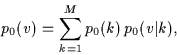
A Bayesian approach
is based on two probability densities:
1. a likelihood model ![]() ,
quantifying the probability of outcome
,
quantifying the probability of outcome ![]() when measuring observable
when measuring observable ![]() given a (not directly observable) potential
given a (not directly observable) potential ![]() and
2. a prior density
and
2. a prior density ![]() =
= ![]() defined over a space
defined over a space ![]() of possible potentials
assuming a priori information
of possible potentials
assuming a priori information ![]() .
Further, let
.
Further, let
![]() =
= ![]() =
=
![]() denote available training data
and
denote available training data
and ![]() =
= ![]() the union of training data and a priori information.
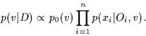
To make predictions
we aim at calculating
the predictive density for given data
the union of training data and a priori information.
To make predictions
we aim at calculating
the predictive density for given data ![]()
According to the axioms of quantum mechanics,
observables ![]() are represented by hermitian operators
and the probability of finding outcome
are represented by hermitian operators
and the probability of finding outcome ![]() measuring observable
measuring observable ![]() is given by
is given by
In particular, we will consider a canonical ensemble of quantum systems
at temperature ![]() (setting Boltzmann's constant to 1)
characterized by the density operator
(setting Boltzmann's constant to 1)
characterized by the density operator
![]() =
=
![]() .
Furthermore, we assume a Hamiltonian
.
Furthermore, we assume a Hamiltonian
![]() =
= ![]() being the sum of a kinetic energy term
being the sum of a kinetic energy term
![]() for a particle with mass
for a particle with mass ![]() and an unknown local potential
and an unknown local potential
![]() =
=
![]() which we want to reconstruct from data.
In case of repeated measurements in a canonical ensemble
one has to wait with the next measurement
until thermal equilibrium is reached again.
We will in the following focus on measurements
of particle coordinates
in a single particle system in a heat bath with temperature
which we want to reconstruct from data.
In case of repeated measurements in a canonical ensemble
one has to wait with the next measurement
until thermal equilibrium is reached again.
We will in the following focus on measurements
of particle coordinates
in a single particle system in a heat bath with temperature ![]() .
In that case the
.
In that case the ![]() represent particle positions
corresponding to measurements of the observable
represent particle positions
corresponding to measurements of the observable ![]() =
= ![]() with
with
![]() =
= ![]() .
The likelihood becomes
.
The likelihood becomes
| (3) |
Already at zero temperature,
even complete knowledge of the true likelihood
would just determine the modulus of the ground state
and thus not be sufficient to determine a potential uniquely.
The situation is still worse in practice,
where only a finite number of probabilistic measurements
is available,
and at finite temperatures,
as the likelihood becomes uniform in the infinite temperature limit.
Hence, in addition to Eq.(2)
giving the likelihood model of quantum mechanics,
it is essential to include
a prior density over a space of possible potentials ![]() .
To be able to formulate a priori information explicitly
in terms of the function values
.
To be able to formulate a priori information explicitly
in terms of the function values ![]() we use a stochastic process.
Technically convenient is a Gaussian process prior
density
we use a stochastic process.
Technically convenient is a Gaussian process prior
density
Typical choices for ![]() implementing smoothness priors
are the negative Laplacian
implementing smoothness priors
are the negative Laplacian
![]() =
= ![]() , e.g.,
in one dimension
, e.g.,
in one dimension ![]() =
= ![]() ,
or a Radial Basis Function prior
,
or a Radial Basis Function prior
![]() =
=
![]() [14].
Gaussian process priors
can, for example, be related to approximate symmetries.
Assume we expect the potential to commute approximately with a
unitary symmetry operation
[14].
Gaussian process priors
can, for example, be related to approximate symmetries.
Assume we expect the potential to commute approximately with a
unitary symmetry operation ![]() . Then
. Then
![]() =
= ![]() defines an operator
defines an operator ![]() acting on potentials
acting on potentials ![]() .
In that case a natural prior would be
.
In that case a natural prior would be
![]() with
with
![]() =
=
![]() =
=
![]() for
for
![]() =
=
![]() and
and ![]() denoting the identity.
Note that symmetric potentials are in the null space of
such a
denoting the identity.
Note that symmetric potentials are in the null space of
such a ![]() ,
hence another prior has to be included
unless the combination with training data does
determine the potential.
Similarly, for a Lie group
,
hence another prior has to be included
unless the combination with training data does
determine the potential.
Similarly, for a Lie group
![]() =
=
![]() an approximate infinitesimal symmetry is implemented by
an approximate infinitesimal symmetry is implemented by
![]() =
=
![]() .
In particular, a negative Laplacian smoothness prior
enforces approximate symmetry under infinitesimal translation.
Alternatively,
a more explicit prior implementing an approximate
symmetry can be obtained by choosing a symmetric reference potential
.
In particular, a negative Laplacian smoothness prior
enforces approximate symmetry under infinitesimal translation.
Alternatively,
a more explicit prior implementing an approximate
symmetry can be obtained by choosing a symmetric reference potential
![]() =
=
![]() and
and ![]() =
=
![]() .
.
While a Gaussian process prior is only able to
model a unimodal, concave prior density,
more general prior densities can be
arbitrarily well approximated by mixtures
of Gaussian process priors [15]
To find the potential with maximal posterior
we maximize for independent data, following Bayes' theorem,
| (10) | |||
It is straightforward to include
also other kinds of data or a priori information.
For example,
a Gaussian smoothness prior as in Eq.(4)
with zero reference potential ![]() and
and ![]() = 0 at the boundaries tends to lead
to flat potentials when the regularization parameters
= 0 at the boundaries tends to lead
to flat potentials when the regularization parameters ![]() becomes large.
For such cases it is useful to include besides smoothness
also a priori information or data
which are related more directly to the depth of the potential.
One such possibility is to include information
about the average energy
becomes large.
For such cases it is useful to include besides smoothness
also a priori information or data
which are related more directly to the depth of the potential.
One such possibility is to include information
about the average energy
![]() =
= ![]() =
=
![]() .
The average energy can then be controled by introducing a Lagrange multiplier
term
.
The average energy can then be controled by introducing a Lagrange multiplier
term
![]() ,
or, technically sometimes easier,
by a term representing noisy energy data
,
or, technically sometimes easier,
by a term representing noisy energy data ![]() ,
,
| (13) |
Collecting all terms we are now able to solve
the stationarity Eq.(7) by iteration.
Starting with an initial guess ![]() ,
choosing a step width
,
choosing a step width ![]() and a positive definite matrix
and a positive definite matrix ![]() we can iterate according to
we can iterate according to
The numerical difficulties of
the nonparametric Bayesian approach
arise from the fact that
the quantum mechanical likelihood (2)
is non-Gaussian and non-local in the potential ![]() .
Similar to general density estimation problems, even for Gaussian priors
none of the
.
Similar to general density estimation problems, even for Gaussian priors
none of the ![]() -integrations in (1)
can be carried out analytically [16].
In contrast, for example,
Gaussian regression problems
have a likelihood being Gaussian and local in the function of interest,
and an analogous nonparametric Bayesian approach
with a Gaussian process prior
requires only to deal with matrices with dimension not larger than
the number of training data [11].
The following examples will show, however,
that a direct numerical solution of Eq.(7)
by discretization is feasible for one-dimensional problems.
Higher dimensional problems, on the other hand,
require further approximations.
For example, work on inverse many-body problems
on the basis of a Hartree-Fock approximation
is in progress.
-integrations in (1)
can be carried out analytically [16].
In contrast, for example,
Gaussian regression problems
have a likelihood being Gaussian and local in the function of interest,
and an analogous nonparametric Bayesian approach
with a Gaussian process prior
requires only to deal with matrices with dimension not larger than
the number of training data [11].
The following examples will show, however,
that a direct numerical solution of Eq.(7)
by discretization is feasible for one-dimensional problems.
Higher dimensional problems, on the other hand,
require further approximations.
For example, work on inverse many-body problems
on the basis of a Hartree-Fock approximation
is in progress.
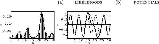 |
In the following numerical examples we discuss
the reconstruction of an approximately periodic,
one-dimensional potential ![]() ,
with the reference potential
,
with the reference potential ![]() chosen periodic.
The potential
chosen periodic.
The potential ![]() may describe a one-dimensional surface,
deviating from exact periodicity due to localized defects.
To enforce the deviation from
may describe a one-dimensional surface,
deviating from exact periodicity due to localized defects.
To enforce the deviation from ![]() to be smooth
we take as prior on
to be smooth
we take as prior on ![]() a negative Laplacian covariance, i.e.,
a negative Laplacian covariance, i.e.,
![]() =
= ![]() .
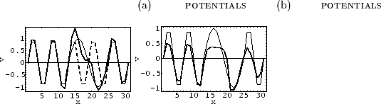
Fig.1 shows representative numerical results
for a grid with 30 points and 200 data sampled
from the likelihood
.
Fig.1 shows representative numerical results
for a grid with 30 points and 200 data sampled
from the likelihood
![]() for some chosen potential
for some chosen potential ![]() .
The reconstructed potential
.
The reconstructed potential ![]() has been found
by iterating without energy penalty term
has been found
by iterating without energy penalty term ![]() according to Eq.(14) with
according to Eq.(14) with
![]() =
= ![]() .
We took zero boundary conditions for
.
We took zero boundary conditions for ![]() ,
so
,
so ![]() becomes invertible,
and, consistently,
periodic boundary conditions for the eigenfunctions
becomes invertible,
and, consistently,
periodic boundary conditions for the eigenfunctions ![]() .
Note that the data have been sufficient to identify clearly
the deviation from the periodic reference potential.
Fig.2a
shows the same example
with an energy penalty term
.
Note that the data have been sufficient to identify clearly
the deviation from the periodic reference potential.
Fig.2a
shows the same example
with an energy penalty term ![]() with
with ![]() =
=
![]() .
While the reconstructed likelihood (not shown) is not much altered,
the true potential is now better approximated in regions where it is small.
As a rule, similar likelihoods do not necessarily imply
similar potentials, and vice versa.
.
While the reconstructed likelihood (not shown) is not much altered,
the true potential is now better approximated in regions where it is small.
As a rule, similar likelihoods do not necessarily imply
similar potentials, and vice versa.
 |
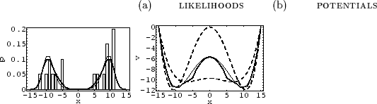 |
Fig.2b
shows the implementation of approximate periodicity
by an operator ![]() ,
defined by
,
defined by
![]() =
=
![]() for periodic boundary conditions on
for periodic boundary conditions on ![]() ,
thus measuring the difference between the potential
,
thus measuring the difference between the potential
![]() and the potential translated by
and the potential translated by ![]() .
To find smooth solutions
we added a negative Laplacian term with zero reference potential, i.e.,
we used
.
To find smooth solutions
we added a negative Laplacian term with zero reference potential, i.e.,
we used
![]() =
=
![]() .
To have an invertible matrix for periodic boundary conditions on
.
To have an invertible matrix for periodic boundary conditions on ![]() we iterated this time with
we iterated this time with
![]() =
= ![]() +
+ ![]() .
The implementation of approximate periodicity by
.
The implementation of approximate periodicity by
![]() instead of a periodic
instead of a periodic ![]() is more general in so far as it annihilates arbitrary functions
with period
is more general in so far as it annihilates arbitrary functions
with period ![]() .
As, however,
the reference function of the Laplacian term does not fit the true
potential very well, the reconstruction is poorer
in regions where the potential is large
and thus no data are available.
In these regions a priori information is of special importance.
Finally, Fig.3
shows the implementation of a mixture of Gaussian prior processes.
.
As, however,
the reference function of the Laplacian term does not fit the true
potential very well, the reconstruction is poorer
in regions where the potential is large
and thus no data are available.
In these regions a priori information is of special importance.
Finally, Fig.3
shows the implementation of a mixture of Gaussian prior processes.
In conclusion, we have applied a nonparametric Bayesian approach to inverse quantum statistics and shown its numerical feasibility for one-dimensional examples.