


Next: Bibliography
Up: Econophysics WS1999/2000: Some Notes
Previous: Linear regression
Finally, we outline the main idea of how portfolios
and spin glasses can be related [3].
This shows that nonlinear constraints can lead to
many solutions for the optimal portfolio.
Consider a portfolio with futures, for
which a margin is required for both sides.
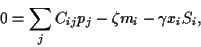
Limiting such margins requires an additional constraint
 |
(46) |
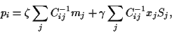
Hence, we may define an optimal portfolio as the minimum of
 |
(47) |
This yields,
 |
(48) |
i.e.,
 |
(49) |
where  = sign
 .
Setting
.
Setting  = 1, and taking the sign yields
![\begin{displaymath}
S_i = {\rm sign} \left[ h_i + \sum_j^N J_{ij}S_j \right]
,
\end{displaymath}](img126.gif) |
(50) |
with  =
=
 and
and  =
=
 .
This is the equation,
for a state which is (locally) stable
under the discrete synchronous Hopfield dynamic,
.
This is the equation,
for a state which is (locally) stable
under the discrete synchronous Hopfield dynamic,
 =
=
![${\rm sign} \left[ h_i + \sum_j J_{ij}S_j \right]$](img132.gif) ,
of a spin glass-like Hamiltonian
,
of a spin glass-like Hamiltonian
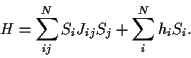 |
(51) |
(For example, in a Hopfield model,
=
 ,
the
,
the  representing patterns to be stored.
In an EA-model (Edwards, Anderson)
the are Gaussian random variables
with distance dependent variance
representing patterns to be stored.
In an EA-model (Edwards, Anderson)
the are Gaussian random variables
with distance dependent variance
 =
=  .
In a SK-model (Sherrington, Kirkpatrick)
the are Gaussian random variables
with distance independent variance
=
.
In a SK-model (Sherrington, Kirkpatrick)
the are Gaussian random variables
with distance independent variance
=  ,
For portfolio theory one can choose
a covariance
,
For portfolio theory one can choose
a covariance  =
=
 built from random matrices
  ,
,  .)
As one knows that the ground state of spin glasses
can be highly degenerated
one can expect a similar effect for such portfolios.
For a random matrix treatment see
[3].
.)
As one knows that the ground state of spin glasses
can be highly degenerated
one can expect a similar effect for such portfolios.
For a random matrix treatment see
[3].
Next: Bibliography
Up: Econophysics WS1999/2000: Some Notes
Previous: Linear regression
Joerg_Lemm
2000-02-25