


Next: Example: Distribution functions
Up: General Gaussian prior factors
Previous: The general case
Contents
Example: Square root of 
We already discussed the cases
 with
with
 ,
,
 and
and  with
with  ,
,
 .
The choice
.
The choice
 yields the common
  -normalization condition over
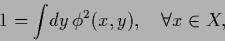 |
(195) |
which is quadratic in  ,
and
,
and  ,
,
 ,
,
 .
For real
the non-negativity condition
.
For real
the non-negativity condition  is automatically
satisfied [82,211].
is automatically
satisfied [82,211].
For =  and a negative Laplacian inverse covariance
  =
=  ,
one can relate the corresponding Gaussian prior
to the Fisher information
[38,211,207].
Consider, for example, a problem with fixed
,
one can relate the corresponding Gaussian prior
to the Fisher information
[38,211,207].
Consider, for example, a problem with fixed  (so can be skipped from the notation and one can write
  )
and a
)
and a  -dimensional .
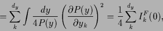
Then one has, assuming the necessary differentiability conditions
and vanishing boundary terms,
-dimensional .
Then one has, assuming the necessary differentiability conditions
and vanishing boundary terms,
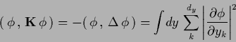 |
(196) |
 |
(197) |
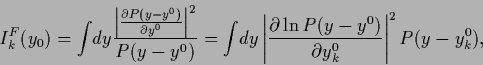
where  is the Fisher information,
defined as
is the Fisher information,
defined as
 |
(198) |
for the family  with location parameter
vector
with location parameter
vector  .
.
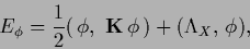
A connection to quantum mechanics can be found
considering the case without training data
 |
(199) |
having the homogeneous stationarity equation
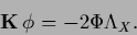 |
(200) |
For -independent  this is an eigenvalue equation.
Examples include the quantum mechanical
Schrödinger equation
where corresponds to the system Hamiltonian
and
this is an eigenvalue equation.
Examples include the quantum mechanical
Schrödinger equation
where corresponds to the system Hamiltonian
and
 |
(201) |
to its ground state energy.
In quantum mechanics Eq. (201) is the basis
for variational methods (see Section 4)
to obtain approximate solutions for ground state energies
[55,197,27].
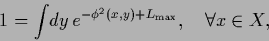
Similarly, one can take
 for
for  bounded from above by
  with the normalization
 |
(202) |
and
 ,
,
 ,
,
 =
=  .
.
Next: Example: Distribution functions
Up: General Gaussian prior factors
Previous: The general case
Contents
Joerg_Lemm
2001-01-21