Trial functions ![]() may be chosen as sum
of simpler functions
may be chosen as sum
of simpler functions ![]() each depending only
on part of the
each depending only
on part of the ![]() and
and ![]() variables.
More precisely, we consider functions
variables.
More precisely, we consider functions ![]() depending on projections
depending on projections ![]() =
=
![]() of the vector
of the vector ![]() =
= ![]() of all
of all ![]() and
and ![]() components.
components.
![]() denotes an projector in the vector space of
denotes an projector in the vector space of
![]() (and not in the space of functions
(and not in the space of functions ![]() ).
Hence,
).
Hence, ![]() becomes of the form
becomes of the form
An ansatz like (391) is made more flexible
by including also interactions
| (394) |
In additive models in the narrower sense
[218,92,93,94]
![]() is a subset of
is a subset of ![]() ,
, ![]() components, i.e.,
components, i.e.,
![]()
![]()
![]() ,
,
![]() denoting the dimension of
denoting the dimension of ![]() ,
,
![]() the dimension of
the dimension of ![]() .
In regression, for example, one takes usually the one-element subsets
.
In regression, for example, one takes usually the one-element subsets
![]() =
= ![]() for
for
![]() .
.
In more general schemes the projections of ![]() do not have to be restricted to projections on the coordinates axes.
In particular, the projections can be optimized too.
For example, one-dimensional projections
do not have to be restricted to projections on the coordinates axes.
In particular, the projections can be optimized too.
For example, one-dimensional projections
![]() =
= ![]() with
with
![]() (where
(where ![]() denotes a scalar product
in the space of
denotes a scalar product
in the space of ![]() variables)
are used by ridge approximation schemes.
They include for regression problems
one-layer (and similarly multilayer)
feedforward neural networks
(see Section 4.9)
projection pursuit regression
(see Section 4.8),
ridge regression [151,152],
and hinge functions [31].
For a detailed discussion of the regression case see
[76].
variables)
are used by ridge approximation schemes.
They include for regression problems
one-layer (and similarly multilayer)
feedforward neural networks
(see Section 4.9)
projection pursuit regression
(see Section 4.8),
ridge regression [151,152],
and hinge functions [31].
For a detailed discussion of the regression case see
[76].
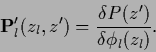
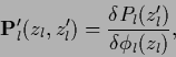
The stationarity equation for ![]() becomes
for the ansatz (391)
becomes
for the ansatz (391)
| (397) |
 |
(398) |
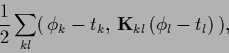 |
(399) |
 |
(400) |
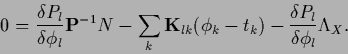
For the parameterized approach (392)
one finds
| (401) |
 |
(402) |