Linearization and Newton algorithm

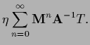
For linear equations ${{\bf K}} \phi$ = $T$ where $T$ and ${{\bf K}}$ are no functions of $\phi$ a spectral radius $\rho ({\bf M})<1$ (the largest modulus of the eigenvalues) of the iteration matrix

$${\bf M} = - \eta {\bf A}^{-1} {\bf B}_\eta =(1-\eta) {\bf I}... ...a {\bf A}^{-1} {\bf B} = {\bf I} - \eta {\bf A}^{-1} {{\bf K}}$$ (631)

would guarantee convergence of the iteration scheme. This is easily seen by solving the linear equation by iteration according to (615)

$$\phi^{(i+1)} = \eta {\bf A}^{-1}T + {\bf M}\phi^{(i)}$$ (632)

$$= \eta {\bf A}^{-1}T + \eta {\bf M} {\bf A}^{-1}T + {\bf M}^2 \phi^{(i-1)}$$ (633)

$$= \eta \sum_{n=0}^\infty {\bf M}^n {\bf A}^{-1} T .$$ (634)

A zero mode of ${{\bf K}}$, for example a constant function for differential operators without boundary conditions, corresponds to an eigenvalue $1$ of ${\bf M}$ and would lead to divergence of the sequence $\phi^{(i)}$. However, a nonlinear $T(\phi)$ or ${{\bf K}}(\phi)$, like the nonlinear normalization constraint contained in $T(\phi)$, can then still lead to a unique solution.

A convergence analysis for nonlinear equations can be done in a linear approximation around a fixed point. Expanding the gradient at $\phi^*$

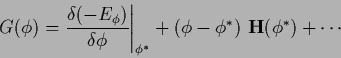$$G(\phi) = \frac{\delta (-E_\phi) }{\delta \phi}\Bigg\vert _{\phi^*} + (\phi-\phi^*) \,\, {\bf H} (\phi^*) + \cdots$$ (635)

shows that the factor of the linear term is the Hessian. Thus in the vicinity of $\phi^*$ the spectral radius of the iteration matrix

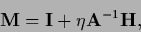$${\bf M} = {\bf I} + \eta {\bf A}^{-1} {\bf H},$$ (636)

determines the rate of convergence. The Newton algorithm uses the negative Hessian $-{\bf H}$ as learning matrix provided it exists and is positive definite. Otherwise it must resort to other methods. In the linear approximation (i.e., for quadratic energy) the Newton algorithm

$${\bf A} = -{\bf H} : {\rm Newton}$$ (637)

is optimal. We have already seen in Sections 3.1.3 and 3.2.3 that the inhomogeneities generate in the Hessian in addition to ${{\bf K}}$ a diagonal part which can remove zero modes of ${{\bf K}}$.