Quadratic concepts

As a first step empirical dependency control requires an explicit and readable formulation of prior knowledge. By explicit formulation we mean in the following the expression of prior knowledge directly in terms of the functions values $h(x)$, like it is done in regularization theory or for stochastic processes. In an implicit implementation of dependencies, on the other hand, single function values $h(x)$ are not parameterized independently. Examples include neural networks, linear, additive or tensor models. Also the realization of learning algorithms can induce dependencies, e.g., due to restricted initial conditions and stopping rules.

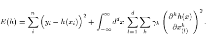
In the regularization framework an approximation $h(x)$ is chosen to minimize a regularization or error functional $E(h)$. Prior knowledge can be represented by a regularization term added to the training error. A typical example of a smoothness related regularization functional for $d$-dimensional $x$ = $\{x_{(1)},\cdots,x_{(d)}\}$ is

$$E(h) = \sum_i^n \Big(y_{i}-h(x_{i})\Big)^2 + \int_{-\infty... ..._k \left( \frac{\partial^k h(x)}{\partial x_{(l)}^k}\right)^2.$$ (1)

It is well known that (for approximation problems with log-loss [5]) a regularization or error functional can be interpreted as up to a constant proportional to the negative logarithm of the posterior probability $p(h\vert D)\propto p(D\vert h)\propto e^{-\beta E(h)}$ with $D=D_T \cup D_P$. For differentiable functionals $E$ the optimal solution $h^*$ is found by setting the functional derivative of $E$ with respect to $h$ to zero. Clearly, the functional $E$ must depend on each single function value $h(x)$ to determine a complete function $h\in {\cal H}$. Thus, for an infinite set ${\cal X}$ the $x$-integral (or a sum over $x$, respectively) corresponds to an infinite number of (prior) data terms. For quadratic terms like in Eq.(1) the common structure of the training data and prior terms can best be seen by writing them as scalar products. Let angular brackets denote scalar products and matrix elements of symmetric operators, e.g. $\mbox{$\left\langle t \vert h \right\rangle$}$ = $\int \!dx\, t(x) h(x)$ and $\mbox{$ \left\langle t\left\vert K\rule[\tiefe]{0cm}{\hoehe} \right\vert h\right\rangle $}$ = $\int \!dx \,dx^\prime t(x)K(x,x^\prime) h(x^\prime)$ = $\mbox{$\left\langle t \vert h \right\rangle$}_K$ where $x$ can be $d$-dimensional. We obtain for a mean-square training error term

$$(y_i-h(x_i))^2 = \int_{-\infty}^\infty \!d^dx \, \delta (x-... ...ule[\tiefe]{0cm}{\hoehe} \right\vert h-t_i\right\rangle $} ,$$

with $t_i\equiv y_i$ and $P_i$ the projector into the space of functions on $x_i$. Similarly, a typical prior term becomes by partial integration for vanishing boundary terms

$$\int_{-\infty}^\infty \!d^dx\, \sum_{l=1}^d \left( \frac{\p... ...ule[\tiefe]{0cm}{\hoehe} \right\vert h-t_0\right\rangle $} ,$$

with $t_0\equiv 0$ and negative (semi) definite $d$-dimensional Laplacian $\Delta$ with kernel $\Delta (x,x^\prime ) = \delta (x-x^\prime)\sum_{l=1}^d \frac{\partial^2}{\partial x_l^2}$. Notice that here, analogously to finite training data $y_i$, a ``continuous data'' or template function function $t_0\equiv 0$ corresponding to infinite data has been introduced explicitly. Indeed, there is no reason except technical convenience why the special function $t_0\equiv 0$ should be preferred over other functions $t(x)$ which are not identically equal to zero. As long as only one continuous data or template function $t(x)$ enters the functional, $t_0\equiv 0$ can always be achieved by solving for $h(x)-t(x)$ instead for $h(x)$. This is possible within classical regularization functionals of the form (1). If, however, more than one template function appears in a functional, then only one of them can be set to zero. Such cases will be studied below. We summarize: Regularization functionals have to contain continuous data (template functions) to determine a function $h$ completely. In the special case of classical functionals of form (1) the template function can be chosen identically zero, so it does not appear explicitly in the formalism. In the general case there is no reason not to consider non-zero template functions. Having motivated the use of continuous data or template functions we now define a quadratic concept. Assume $h$ to be in some Hilbert space ${\cal H}$.

Definition. (Quadratic concept.) A quadratic concept is a pair $(t,K)$ consisting of a template function $t(x)\in {\cal H}$ and a real symmetric, positive semi-definite operator on ${\cal H}$, the concept operator $K$. The operator $K$ defines a concept distance $d^2 (h) = \mbox{$ \left\langle h-t\left\vert K\rule[\tiefe]{0cm}{\hoehe} \right\vert h-t\right\rangle $} = \vert\vert h-t\vert\vert^2_{K}$ on subspaces where it is positive definite. The maximal subspace in which the positive semi-definite $K$ is positive definite is the concept space $H_K$ of $K$. The corresponding hermitian projector $P_K$ in this subspace $H_K$ is the concept projector.

Remark 1 (Approximate symmetries): Typical concept operators $K$ are related to symmetries. Let for example $Sh(x) = h(\sigma(x))$ with $\sigma$ a permutation within ${\cal X}$, i.e., one-to-one. Then $K$ = $(I-S)^T(I-S)$, with identity $I$ and ${}^T$ denoting the transpose, defines a symmetry concept $d_S^2 (h) = \mbox{$\left\langle h-Sh \vert h-Sh \right\rangle$}$. Similarly, assume $S(\theta)=e^{\theta s}$ to be a continuous symmetry (Lie) group, parameterized by $\theta$ and with infinitesimal generators $s$. Then an infinitesimal symmetry concept for $S\approx 1+\theta s$ is defined by $d_s^2(h) = \mbox{$\left\langle sh \vert sh \right\rangle$}$. For infinitesimal translations (smoothness) $s=\partial/\partial x$.

Remark 2 (Gaussian processes): A quadratic concept defines a Gaussian process according to $p(D\vert h) \propto e^{-d^2(h)/2}$ with covariance operator $K^{-1}$. We remark however, that while Gaussian processes can also be defined for continuous ${\cal X}$ [2,7] we do not discuss continuum limits for the non-Gaussian extensions below. In these cases we refer to a lattice approximation.

Remark 3 (Support vector machine): Expanding $h=\sum_m n_m \Phi_m(x)$ in a basis of eigenfunctions of $K=\sum_m \lambda_m \Phi_m \Phi_m^T$ one obtains $E(h) =\sum_i\big( y_i-h(x_i)\big )^2+\mbox{$ \left\langle h\left\vert K\rule[\tiefe]{0cm}{\hoehe} \right\vert h\right\rangle $}$ = $\sum_i \left( \sum_m n_m \Phi_m(x)-y_i\right)^2+\lambda_m \vert n_m\vert^2$. Replacing the mean-square training error by Vapnik's $\epsilon$-insensitive error yields a support vector machine with kernel $K$ [6]. In general, flat regions of $E(h)$ as they appear in the $\epsilon$-insensitive error and other robust error functions have the technical advantage that they do not contribute to the gradient and can be ignored within a saddle point approximation.

Remark 4 (Templates): Templates $t(x)$ can be constructed directly by experts. They also can represent a structural hypothesis realized by a parameterized learning system like a neural network. Templates can be used for transfer by choosing them as the output of a learning system trained for a similar situation. For finite spaces templates can in principle be estimated by sampling.

Remark 5 (Covariances): Covariances $K^{-1}$ can be given directly by experts. They do not necessarily have to be local but can include non-local correlations. As already remarked they are often constructed from symmetry considerations. For finite spaces covariances can in principle also be estimated by sampling.