Next: Capital Asset Pricing Model
Up: Econophysics WS1999/2000: Some Notes
Previous: Introduction
Following the discussion of
optimal portfolios for uncorrelated assets
in the last lecture,
we study now portfolios of correlated assets.
Let again be
 = number of assets,
 = value of riskless asset,
 = value of risky asset
  ,
,  , and
, and
 = number of assets of kind .
Investing in a portfolio
with initial wealth
 |
(1) |
at some later time  the wealth of portfolio will be
 |
(2) |
For convenience, we take again
 = 1,
= 1,  = 1,
i.e.,
= 1,
i.e.,  = so that
the condition
= so that
the condition
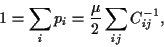
 = 1 must hold.
To be specific, we will now asssume
the  to be Gaussian random variables
 |
(3) |
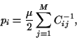
The real symmetric, positive definite covariance matrix  can be diagonalized
by an orthogonal transformation
can be diagonalized
by an orthogonal transformation  =
=  .
Thus, the asset combinations
.
Thus, the asset combinations  defined by
 |
(4) |
are uncorrelated.
In particular, we assume
the expected returns of asset
 |
(5) |
to be known.
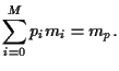
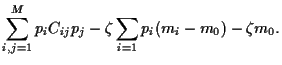
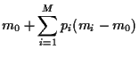
Hence, the expected return of portfolio is the linear combination
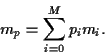 |
(6) |
Furthermore, we also assume the covariance matrix  of assets
to be known
of assets
to be known
This is a nontrivial assumption, as guesses for covariances
are difficult to obtain in practice.
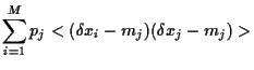
Similarly, we find for the covariance
between asset and the portfolio 
and finally
for the variance of portfolio
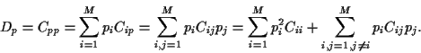 |
(13) |
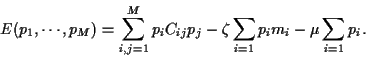
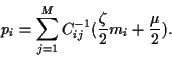
The main idea of Markowitz was to find an optimal portfolio
by minimizing its variance  fixing its expected return
  .
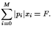
Minimizing must be done under some constraints.
Necessary constraints are
.
Minimizing must be done under some constraints.
Necessary constraints are
Note, that some might be negative
if short selling of assets is allowed.
Other possible constraints,
describing specific situations, can be, for example,
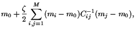
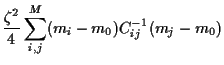
Example 1:
Minimize portfolio variance subject to
(i)
=  and (ii)
 = .
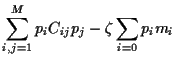
Implementing the first constraint explicitly
and introducing a Lagrange multiplier
= .
Implementing the first constraint explicitly
and introducing a Lagrange multiplier  for the second
results in
for the second
results in
It follows from
 = 0 for
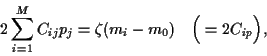 |
(22) |
and thus, inverting the covariance
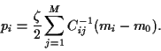 |
(23) |
The Lagrange multiplier is obtained from
i.e.,
 |
(27) |
For we find
hence
 |
(31) |
Example 2:
Minimize portfolio variance without riskless asset
subject to
(i)
=
and (ii)
= .
Implementing the both constraints
by introducing Lagrange multiplier and  results in
 |
(32) |
It follows from
= 0 for
 |
(33) |
The point with the lowest risk has  = 0, so that
 |
(34) |
and for follows
 |
(35) |
i.e.,
 |
(36) |
All optimal portfolios must have more risk.
For the general case the Lagrange multipliers  and
can be obtained similarly as in Example 1.
and
can be obtained similarly as in Example 1.
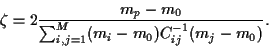
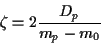
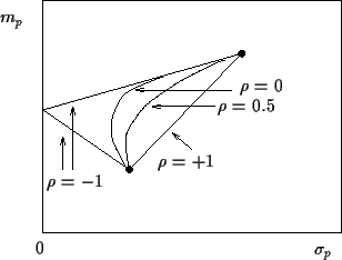
Fig. 1 shows the dependency of
a portfolio of two risky assets
from their correlation coefficient.
The correlation coefficient, defined
as  =
=
 .
=
.
=
 ,
can only take values between
,
can only take values between  (perfect anti-correlation)
and
(perfect anti-correlation)
and  (perfect correlation).
In the extreme case of perfect
anti-correlation, i.e.,
= ,
the two risky assets can be combined to a
riskfree portfolio.
If one of the two assets is riskfree,
all the straight lines in the figure coincide (see example 1).
(perfect correlation).
In the extreme case of perfect
anti-correlation, i.e.,
= ,
the two risky assets can be combined to a
riskfree portfolio.
If one of the two assets is riskfree,
all the straight lines in the figure coincide (see example 1).
Figure 1:
Portfolios of two risky correlated assets
without short selling
in the - plane.
 |
Next: Capital Asset Pricing Model
Up: Econophysics WS1999/2000: Some Notes
Previous: Introduction
Joerg_Lemm
2000-02-25