Capital Asset Pricing Model (CAPM)

Inserting Eq. (31) into Eq. (22) results in a relation between $m_i$ and $m_p$,

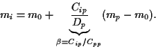$$m_i = m_0 + \underbrace{\frac{C_{ip}}{D_p}}_{\beta=C_{ip}/C_{pp}}(m_p-m_0).$$ (37)

(known as security market line) or, in terms of the standard deviation $\sigma _p$ = $\sqrt{D_p}$,

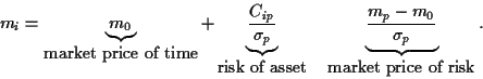$$m_i = \underbrace{m_0}_{\mbox{market price of time}} + \un... ...brace{\frac{m_p-m_0}{\sigma_p}}_{\mbox{market price of risk}}.$$ (38)

The Capital Asset Pricing Model (CAPM) assumes that all agents use this mean variance portfolio with the same guesses for $m_i$ and $D_i$. It follows that the whole market can be considered as a mean variance portfolio, the so called market portfolio. Furthermore, the only free parameter of a rational investor should be the proportion $p_0$ of the riskless asset which is mixed with the market portfolio. I.e, letting $m_p$ denote the expected return of the market portfolio, individual portfolios with returns $m_i$ are on the line

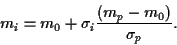$$m_i = m_0 + \sigma_i \frac{(m_p-m_0)}{\sigma_p}.$$ (39)

(capital market line) parametrized by $\sigma_i$ [2]. Much empirical work has been devoted to check the validity of the CAPM with differing results.