Let us consider prior densities
being a product of a Gaussian
prior ![]() as in Eq. (34),
or more general a mixture of Gaussian processes as in
Eq. (40),
and a non-Gaussian energy prior
as in Eq. (34),
or more general a mixture of Gaussian processes as in
Eq. (40),
and a non-Gaussian energy prior
![]() of the form
of Eq. (43).
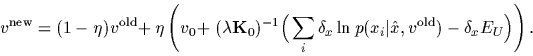
In that case, the stationarity equation we have to solve
to maximize the posterior density of Eq. (33)
reads
of the form
of Eq. (43).
In that case, the stationarity equation we have to solve
to maximize the posterior density of Eq. (33)
reads
| (45) |
 |
(46) |
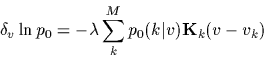
To get the functional derivative of the non-Gaussian ![]() we calculate first
we calculate first
| (47) |
| (48) |
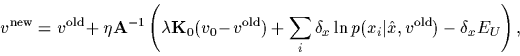
Collecting all terms, we can now solve
the stationarity equation (44)
by iteration
A simple and useful choice in our case is
![]() =
= ![]() which approximates the Hessian.
For a single Gaussian prior
this choice does
not depend on
which approximates the Hessian.
For a single Gaussian prior
this choice does
not depend on ![]() and has thus not to be recalculated during iteration.
Eq. (49) then becomes
and has thus not to be recalculated during iteration.
Eq. (49) then becomes
Due to the nonparametric approach for the potential combined with a priori information implemented as stochastic process, the Bayesian approach formulated in the previous sections is clearly computationally demanding. The situation for inverse quantum theory is worse than, e.g., for Gaussian process priors in regression problems (i.e., for a Gaussian likelihood, local in the regression function) where it is only necessary to work with matrices having a dimension equal to the number of training data [16,48]. In our case, where the likelihood is nonlocal in the potential and also non-Gaussian prior terms may occur, the stationarity equation has to be solved be discretizing the problem.
The following section demonstrates
that at least one-dimensional problems
can be solved numerically
without further approximation.
Higher dimensional problems, however, e.g., for many-body systems,
require additional approximations.
In such higher dimensional situations,
the potential may be parameterized
(without skipping necessarily the prior terms)
or the problem has to be divided
in lower dimensional subproblems, e.g.,
by restricting ![]() to certain
(typically, additive or multiplicative)
combinations of lower dimensional functions.
(Similarly, for example to
additive models [19]
projection pursuit [20]
or neural network like
[22]
approaches.)
to certain
(typically, additive or multiplicative)
combinations of lower dimensional functions.
(Similarly, for example to
additive models [19]
projection pursuit [20]
or neural network like
[22]
approaches.)