Next: Integer hyperparameters
Up: Parameterizing priors: Hyperparameters
Previous: Regularization parameters
Contents
In the previous sections we have studied saddle point approximations
which lead us to maximize the joint posterior
 simultaneously with respect to the hidden variables
  and
and 
 |
(486) |
assuming for the maximization with respect to
a slowly varying  at the stationary point.
This simultaneous maximization with respect to both variables
is consistent with the usual asymptotic
justification of a saddle point approximation.
For example, for a function  of two
(for example, one-dimensional)
variables ,
of two
(for example, one-dimensional)
variables ,
 |
(487) |
for large enough  (and a unique maximum).
Here
(and a unique maximum).
Here
 denotes the joint minimum
and
denotes the joint minimum
and  the Hessian of
  with respect to and .
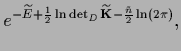
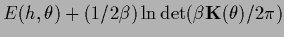
For -dependent determinant of the covariance
and the usual definition of ,
results in a function of the form
=
with respect to and .
For -dependent determinant of the covariance
and the usual definition of ,
results in a function of the form
=
 ,
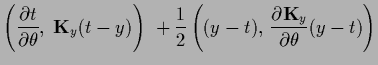
where both terms are relevant for
the minimization of with respect to .
For large , however, the second term
becomes small compared to the first one.
(Of course, there is the possibility that a saddle point approximation
is not adequate for the integration.
Also, we have seen
that the condition of a positive definite covariance
may lead to a solution for on the boundary
where the (unrestricted) stationarity equation is not fulfilled.)
,
where both terms are relevant for
the minimization of with respect to .
For large , however, the second term
becomes small compared to the first one.
(Of course, there is the possibility that a saddle point approximation
is not adequate for the integration.
Also, we have seen
that the condition of a positive definite covariance
may lead to a solution for on the boundary
where the (unrestricted) stationarity equation is not fulfilled.)
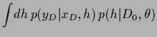
Alternatively,
one might think of performing the two integrals stepwise.
This seems especially useful if one integral
can be calculated analytically.
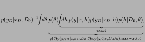
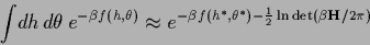
Consider, for example
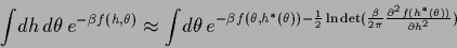 |
(488) |
which would be exact for a Gaussian -integral.
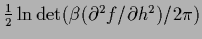
One sees now that
minimizing the complete negative exponent
 +
+
 with respect to
is different from minimizing only in (487),
if the second derivative of with respect to depends on
(which is not the case for a Gaussian integral).
Again this additional term becomes negligible for large enough .
Thus, at least asymptotically,
this term may be altered or even be skipped,
and differences in the results of
the variants of saddle point approximation
will be expected to be small.
with respect to
is different from minimizing only in (487),
if the second derivative of with respect to depends on
(which is not the case for a Gaussian integral).
Again this additional term becomes negligible for large enough .
Thus, at least asymptotically,
this term may be altered or even be skipped,
and differences in the results of
the variants of saddle point approximation
will be expected to be small.
Stepwise approaches like (488) can be used, for example
to perform Gaussian integrations analytically,
and lead to somewhat simpler
stationarity equations for -dependent covariances
[236].
In particular,
let us look at
the case of Gaussian regression in a bit more detail.
The following discussion, however, also applies
to density estimation if, as in (488),
the Gaussian first step integration is replaced
by a saddle point approximation including the normalization factor.
(This requires the calculation of the determinant of the Hessian.)
Consider the two step procedure for Gaussian regression
where in a first step
 can be calculated
analytically and in a second step the integral is performed
by Gaussian approximation around a stationary point.
Instead of maximizing
the joint posterior
with respect to and
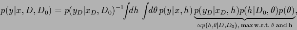
this approach performs the -integration analytically and maximizes
can be calculated
analytically and in a second step the integral is performed
by Gaussian approximation around a stationary point.
Instead of maximizing
the joint posterior
with respect to and
this approach performs the -integration analytically and maximizes
 with respect to .
The disadvantage of this approach
is the
with respect to .
The disadvantage of this approach
is the  -, and
  -dependency of the resulting solution.
Thus,
assuming a slowly varying
 at the stationary point
it appears simpler to
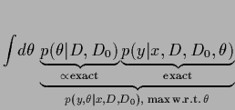
maximize the -marginalized
posterior,
at the stationary point
it appears simpler to
maximize the -marginalized
posterior,
 =
=
 ,
if the -integration can be performed exactly,
,
if the -integration can be performed exactly,
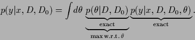 |
(490) |
Having found a maximum posterior solution  the corresponding analytical solution
for
the corresponding analytical solution
for
 is then given by Eq. (321).
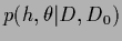
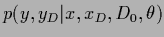
The posterior density
can be obtained from the likelihood of
and a specified prior
is then given by Eq. (321).
The posterior density
can be obtained from the likelihood of
and a specified prior 
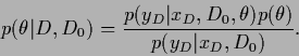 |
(491) |
Thus, in case the -likelihood can be calculated
analytically,
the -integral is calculated in saddle point approximation
by maximizing the posterior for
with respect to .
In the case of a uniform
the optimal is obtained
by maximizing the -likelihood.
This corresponds technically to an empirical Bayes approach
[35].
As is integrated out in
 the -likelihood is also called
marginalized likelihood.
the -likelihood is also called
marginalized likelihood.
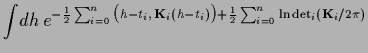
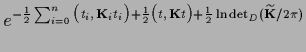
Indeed, for Gaussian regression,
the -likelihood
can be integrated analytically.
Analogously to Section 3.7.2 one finds
[228,237,236],
where
 =
=
 ,
,
 =
=
 =
=
 ,
,
 the determinant in data space,
and we used that
from
the determinant in data space,
and we used that
from
 =
=  for
for  follows
 =
=
 +
+
 =
=
 ,
with
,
with
 =
=
 .
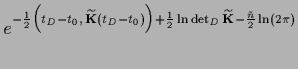
In cases where the marginalization over ,
necessary to obtain the evidence,
cannot be performed analytically
and all -integrals are calculated in saddle point approximation,
we get the same result as
for a direct simultaneous MAP for and
for the predictive density
as indicated in (486).
.
In cases where the marginalization over ,
necessary to obtain the evidence,
cannot be performed analytically
and all -integrals are calculated in saddle point approximation,
we get the same result as
for a direct simultaneous MAP for and
for the predictive density
as indicated in (486).
Now we are able to compare the three
resulting stationary equations for
-dependent mean  ,
inverse covariance
,
inverse covariance
 and prior .
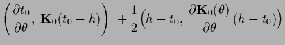
Setting the derivative of the joint posterior
with respect to
to zero yields
and prior .
Setting the derivative of the joint posterior
with respect to
to zero yields
This equation which we have already discussed
has to be solved simultaneously with the stationarity equation
for .
While this approach is easily adapted
to general density estimation problems,
its difficulty for -dependent covariance determinants
lies in calculation of the derivative of the determinant of  .
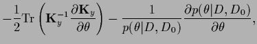
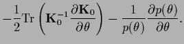
Maximizing the -marginalized posterior
,
on the other hand,
only requires
the calculation of the derivative of the determinant of the
.
Maximizing the -marginalized posterior
,
on the other hand,
only requires
the calculation of the derivative of the determinant of the
 matrix
Evaluated
at the stationary
 =
=
 ,
the first term of Eq. (493),
which does not contain derivatives of the inverse covariances,
becomes equal to the first term of Eq. (494).
The last terms of
Eqs. (493) and (494)
are always identical.
Typically, the data-independent
has a more regular structure
than the data-dependent
.
Thus,
at least for one or two dimensional ,
a straightforward numerical solution of Eq. (493)
by discretizing
can also be a good choice for Gaussian regression problems.
,
the first term of Eq. (493),
which does not contain derivatives of the inverse covariances,
becomes equal to the first term of Eq. (494).
The last terms of
Eqs. (493) and (494)
are always identical.
Typically, the data-independent
has a more regular structure
than the data-dependent
.
Thus,
at least for one or two dimensional ,
a straightforward numerical solution of Eq. (493)
by discretizing
can also be a good choice for Gaussian regression problems.
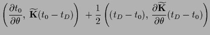
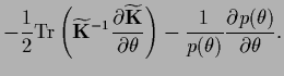
Analogously, from Eq. (321) follows
for maximizing
with respect to
which is -, and -dependent.
Such an approach may be considered
if interested only in specific test data , .
We may remark that also in Gaussian regression the -integral
may be quite different from a Gaussian integral,
so a saddle point approximation
does not necessarily have to give satisfactory results.
In cases one encounters problems one can, for example, try
variable transformations
 =
=
 to obtain a more Gaussian shape of the integrand.
Due to the presence of the Jacobian determinant, however,
the asymptotic interpretation of the corresponding saddle point approximation
is different for the two integrals.
The variability of saddle point approximations
results from the freedom to add terms which vanish
asymptotically but remains finite in the nonasymptotic region.
Similar effects are known in quantum many body theory
(see for example [172], chapter 7.)
Alternatively, the -integral can be solved numerically
by Monte Carlo methods[237,236].
to obtain a more Gaussian shape of the integrand.
Due to the presence of the Jacobian determinant, however,
the asymptotic interpretation of the corresponding saddle point approximation
is different for the two integrals.
The variability of saddle point approximations
results from the freedom to add terms which vanish
asymptotically but remains finite in the nonasymptotic region.
Similar effects are known in quantum many body theory
(see for example [172], chapter 7.)
Alternatively, the -integral can be solved numerically
by Monte Carlo methods[237,236].
Next: Integer hyperparameters
Up: Parameterizing priors: Hyperparameters
Previous: Regularization parameters
Contents
Joerg_Lemm
2001-01-21