Next: Gaussian mixture regression (cluster
Up: Regression
Previous: Gaussian regression
Contents
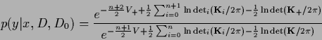
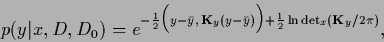
Exact predictive density
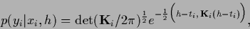
For Gaussian regression the predictive density
under training data  and prior
  can be found analytically
without resorting to a saddle point approximation.
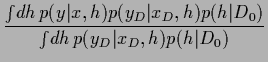
The predictive density is defined as the
can be found analytically
without resorting to a saddle point approximation.
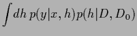
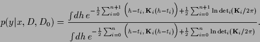
The predictive density is defined as the  -integral
Denoting
training data values  by
by  sampled with inverse covariance
  concentrated on
  and analogously
test data values
and analogously
test data values  =
=  by
by  sampled with inverse (co-)variance
  ,
we have for
,
we have for 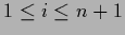
 |
(308) |
and
 |
(309) |
hence
 |
(310) |
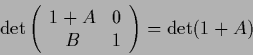
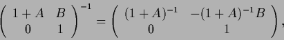
Here we have this time written explicitly
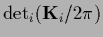 for a determinant calculated
in that space where
for a determinant calculated
in that space where  is invertible.
This is useful because for example in general
is invertible.
This is useful because for example in general
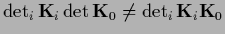 .
Using the generalized `bias-variance'-decomposition (230)
yields
.
Using the generalized `bias-variance'-decomposition (230)
yields
 |
(311) |
with
Now the  -integration can be performed
 |
(316) |
Canceling common factors,
writing again for ,
 for ,
for ,
 for
for  ,
and
using
,
and
using
 =
=
 ,
this becomes
,
this becomes
 |
(317) |
Here we introduced
 =
=  =
=
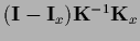
 and used that
 |
(318) |
can be calculated in the space of test data  .
This follows from
.
This follows from
 =
=
 and the equality
 |
(319) |
with
 =
=
 ,
,
 =
=
 ,
and
,
and  denoting the projector
into the space of test data .
Finally
denoting the projector
into the space of test data .
Finally
 |
(320) |
yields the correct normalization of the predictive density
 |
(321) |
with mean and covariance
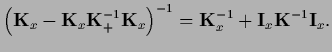
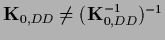
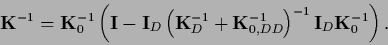
It is useful to express
the posterior covariance  by
the prior covariance
by
the prior covariance
 .
According to
.
According to
 |
(324) |
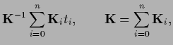
with
=
 ,
=
,
=
 ,
and
,
and
 =
=
 ,
,
 =
=
 ,
,
 =
=
 we find
Notice that while
 =
=
 in general
=
in general
=
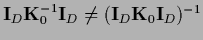 .
This means for example that
.
This means for example that
 has to be
known to find
and it is not enough to invert
has to be
known to find
and it is not enough to invert
 =
=
 .
In data space
.
In data space
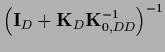 =
=
 ,
so Eq. (325) can be manipulated to give
,
so Eq. (325) can be manipulated to give
 |
(326) |
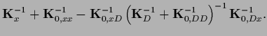
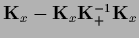
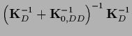
This allows now to express
the predictive mean (322) and covariance (323)
by the prior covariance
Thus, for given prior covariance
both,
 and
and
 ,
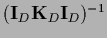
can be calculated
by inverting the
,
can be calculated
by inverting the
 matrix
 =
=
 .
.
Comparison of Eqs.(327,328)
with the maximum posterior solution  of
Eq. (277)
now shows that for Gaussian regression
the exact predictive density
of
Eq. (277)
now shows that for Gaussian regression
the exact predictive density
 and its
maximum posterior approximation
and its
maximum posterior approximation
 have the same
mean
have the same
mean
 |
(329) |
The variances, however, differ
by the term
 .
.
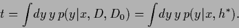
According to the results of Section 2.2.2
the mean of the predictive density
is the optimal choice under squared-error loss (51).
For Gaussian regression, therefore
the optimal regression function
 is the same for squared-error loss
in exact and in maximum posterior treatment
and thus also for log-loss
(for Gaussian
is the same for squared-error loss
in exact and in maximum posterior treatment
and thus also for log-loss
(for Gaussian  with fixed variance)
 |
(330) |
In case the space of possible
is not restricted to Gaussian densities with fixed variance,
the variance of the optimal density under log-loss
 = differs by
from its maximum posterior approximation
= differs by
from its maximum posterior approximation
 = .
= .
Next: Gaussian mixture regression (cluster
Up: Regression
Previous: Gaussian regression
Contents
Joerg_Lemm
2001-01-21