Next: Non-quadratic potentials
Up: Non-Gaussian prior factors
Previous: Analytical solution of mixture
Contents
Local mixtures
Global mixture components can be obtained
by combining local mixture components.
Predicting a time series, for example,
one may allow to switch locally (in time)
between two or more possible regimes,
each corresponding to a different local covariance or template.
The problem which arises when combining local alternatives
is the fact that
the total number of mixture components
grows exponentially in the number local components
which have to be combined
for a global mixture component.
Consider a local prior mixture model,
similar to Eq. (531),
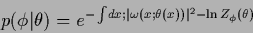 |
(588) |
where  may be a binary or an integer variable.
The local mixture variable
labels local alternatives for filtered differences
may be a binary or an integer variable.
The local mixture variable
labels local alternatives for filtered differences
 which may differ in
their templates
which may differ in
their templates
 and/or
their local filters
and/or
their local filters
 .
To avoid infinite products,
we choose a discretized
.
To avoid infinite products,
we choose a discretized  variable (which may include
the
variable (which may include
the  variable for general density estimation problems),
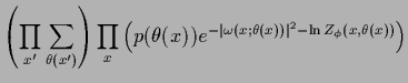
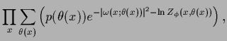
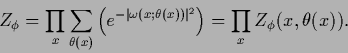
so that
variable for general density estimation problems),
so that
 |
(589) |
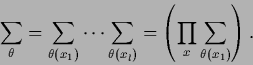
where the sum  is over all local integer variables , i.e.,
 |
(590) |
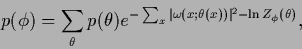
Only for factorizing hyperprior
 =
=
 the complete posterior factorizes
because
 |
(592) |
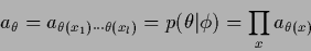
Under that condition the mixture coefficients  of Eq. (552)
can be obtained from the equations,
local in ,
of Eq. (552)
can be obtained from the equations,
local in ,
 |
(593) |
with
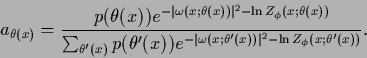 |
(594) |
For equal covariances this is a nonlinear equation
within a space of dimension equal to the number of local components.
For non-factorizing hyperprior
the equations for different
cannot be decoupled.
Next: Non-quadratic potentials
Up: Non-Gaussian prior factors
Previous: Analytical solution of mixture
Contents
Joerg_Lemm
2001-01-21