Next: Non-Gaussian prior factors
Up: Parameterizing priors: Hyperparameters
Previous: Integer hyperparameters
Contents
Local hyperfields
Most, but not all hyperparameters  considered so far have been real or integer numbers,
or vectors with real or integer components
considered so far have been real or integer numbers,
or vectors with real or integer components  .
With the unrestricted template functions of Sect. 5.2.3
or the functions parameterizing the inverse covariance
in Section 5.3.3,
we have, however, also already encountered
function hyperparameters or hyperfields.
In this section we will now discuss
function hyperparameters in more detail.
.
With the unrestricted template functions of Sect. 5.2.3
or the functions parameterizing the inverse covariance
in Section 5.3.3,
we have, however, also already encountered
function hyperparameters or hyperfields.
In this section we will now discuss
function hyperparameters in more detail.
Functions can be seen as continuous vectors,
the function values  being the (continuous) analogue of vector components .
In numerical calculations, in particular,
functions usually have to be discretized,
so, numerically, functions stand for high dimensional vectors.
being the (continuous) analogue of vector components .
In numerical calculations, in particular,
functions usually have to be discretized,
so, numerically, functions stand for high dimensional vectors.
Typical arguments of function hyperparameters
are the independent variables  and, for general density estimation, also the dependent variables
  .
Such functions
.
Such functions  or
or  will be called
local hyperparameters or local hyperfields.
Local hyperfields
can be used, for example,
to adapt templates or inverse covariances locally.
(For general density estimation problems
replace here and in the following by
will be called
local hyperparameters or local hyperfields.
Local hyperfields
can be used, for example,
to adapt templates or inverse covariances locally.
(For general density estimation problems
replace here and in the following by  .)
.)
The price to be paid for the additional flexibility
of function hyperparameters
is a large number of additional degrees of freedom.
This can considerably complicate calculations and,
requires a sufficient number of training data
and/or a sufficiently restrictive hyperprior
to be able to determine the hyperfield
and not to make the prior useless.
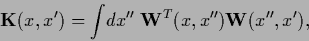
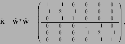
To introduce local hyperparameters
we express real symmetric, positive (semi-)definite inverse covariances
by square roots or ``filter operators''  ,
,
 =
=
 =
=
 where
where
 represents the vector
 .
Thus, in components
.
Thus, in components
 |
(498) |
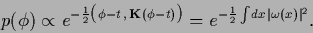
and therefore
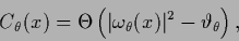
where we defined the ``filtered differences''
![\begin{displaymath}
\omega (x)
=
\big( \, W_x\, ,\, \phi-t \, \big)
=
\int \!dx^\prime \, {\bf W}(x,x^\prime)
[\phi(x^\prime)-t(x^\prime )]
.
\end{displaymath}](img1751.png) |
(500) |
Thus, for a Gaussian prior for  we have
 |
(501) |
A real local hyperfield
mixing, for instance,
locally two alternative filtered differences
may now be introduced as follows
 |
(502) |
where
![\begin{displaymath}
\omega (x;\theta)
= [1-\theta(x)] \, \omega_1(x) + \theta(x) \,\omega_2(x)
,
\end{displaymath}](img1754.png) |
(503) |
and, say,
![$\theta(x)\in [0,1]$](img1755.png) .
For unrestricted real
an arbitrary real
.
For unrestricted real
an arbitrary real
 can be obtained.
For a binary local hyperfield
with
can be obtained.
For a binary local hyperfield
with
 we have
 = ,
= ,
 =
=  ,
and
,
and
 =
=  ,
so
Eq. (502)
becomes
,
so
Eq. (502)
becomes
 |
(504) |
For real
in Eq. (503)
terms with  ,
,
![$[1-\theta(x)]^2$](img1764.png) , and
, and
![$[1-\theta(x)]\theta(x)$](img1765.png) would appear in Eq. (504).
A binary variable can
be obtained from a real
with the help of a step function
would appear in Eq. (504).
A binary variable can
be obtained from a real
with the help of a step function  and a threshold
  by replacing
 |
(505) |
Clearly, if both prior and hyperprior are formulated
in terms of such  this is equivalent to using directly a binary hyperfield.
For a local hyperfield
a local adaption of the functions
as in Eq. (503)
can be achieved by switching
locally between alternative templates
or alternative filter operators
In Eq. (506)
it is important to notice that ``local'' templates
 for fixed
are still functions
of an
for fixed
are still functions
of an  variable.
Indeed, to obtain
,
the function
variable.
Indeed, to obtain
,
the function  is needed for all for which
has nonzero entries,
is needed for all for which
has nonzero entries,
![\begin{displaymath}
\omega(x;\theta )
=
\int\!dx^\prime\,
{\bf W}(x,x^\prime)
[\phi(x^\prime)-t_x(x^\prime;\theta)]
.
\end{displaymath}](img1777.png) |
(508) |
That means that the template
is adapted individually for every local filtered difference.
Thus, Eq. (506)
has to be distinguished from the choice
![\begin{displaymath}
t(x^\prime;\theta)
=
[1-\theta(x^\prime )] \, t_{1}(x^\prime)
+ \theta(x^\prime )\, t_{2}(x^\prime)
.
\end{displaymath}](img1778.png) |
(509) |
The unrestricted adaption of templates
discussed in Sect. 5.2.3,
for instance,
can be seen as an approach of the form of
Eq. (509)
with an unbounded real hyperfield .
Eq. (507)
corresponds
for binary to an inverse covariance
 |
(510) |
where
 =
=
 and
and
 =
=
 ,
,
 =
=
 .
We remark that -dependent inverse covariances
require to include the normalization factors
when integrating over or
solving for the optimal in MAP.
If we consider
two binary hyperfields ,
.
We remark that -dependent inverse covariances
require to include the normalization factors
when integrating over or
solving for the optimal in MAP.
If we consider
two binary hyperfields ,  ,
one for
,
one for  and one for ,
we get a prior
and one for ,
we get a prior
![\begin{displaymath}
p(\phi\vert\theta,\theta^\prime)
\propto
e^{-\frac{1}{2}
\in...
...theta)]\big)
}
\propto
e^{-E(\phi\vert\theta,\theta^\prime)}
.
\end{displaymath}](img1787.png) |
(511) |
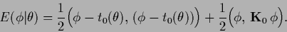
Up to a -independent constant
(which still depends on , )
the corresponding prior energy
can again be written in the form
![\begin{displaymath}
E(\phi\vert\theta,\theta^\prime)
=
\frac{1}{2}
\Big( \phi-t(...
...{\bf K}(\theta^\prime ) [\phi-t(\theta,\theta^\prime)] \Big)
.
\end{displaymath}](img1788.png) |
(512) |
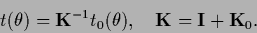
Indeed,
the corresponding effective template
 and effective inverse covariance
 are according to Eqs. (247,252)
given by
are according to Eqs. (247,252)
given by
Hence, one may rewrite
The MAP solution of Gaussian regression
for a prior corresponding to (515)
at optimal  ,
,
 is according to Section 3.7
therefore
given by
is according to Section 3.7
therefore
given by
 |
(516) |
One may avoid dealing with
``local'' templates  by adapting templates
in prior terms where is equal to the identity
by adapting templates
in prior terms where is equal to the identity  .
In that case
.
In that case
 is only needed for =
and we may thus directly write
=
is only needed for =
and we may thus directly write
=
 .
As example, consider the following prior energy,
where the -dependent template
is located in a term with =
and another, say smoothness, prior is added
with zero template
.
As example, consider the following prior energy,
where the -dependent template
is located in a term with =
and another, say smoothness, prior is added
with zero template
 |
(517) |
Combining both terms yields
 |
(518) |
with effective template and effective inverse covariance
 |
(519) |
For differential operators
the effective  is thus a smoothed version of
  .
.
The extreme case would be to treat
and itself as unrestricted hyperparameters.
Notice, however, that increasing flexibility tends to lower
the influence of the corresponding prior term.
That means,
using completely free templates and covariances
without introducing additional restricting hyperpriors,
just eliminates the corresponding prior term
(see Section 5.2.3).
Hence, to restrict the flexibility,
typically a smoothness hyperprior may be imposed
to prevent highly oscillating functions .
For real , for example, a smoothness prior
like
 can be used
in regions where it is defined.
(The space of -functions
for which a smoothness prior
can be used
in regions where it is defined.
(The space of -functions
for which a smoothness prior
 with discontinuous is defined
depends on the locations of the discontinuities.)
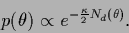
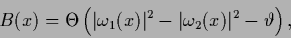
An example of a non-Gaussian hyperprior is,
with discontinuous is defined
depends on the locations of the discontinuities.)
An example of a non-Gaussian hyperprior is,
 |
(520) |
where  is some constant
and
is some constant
and
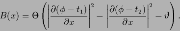
 |
(521) |
is zero at locations where the square of the first derivative
is smaller than a certain
threshold
 ,
and one otherwise.
(The step function
,
and one otherwise.
(The step function  is defined as = 0 for
  and = 1 for
  .)
To enable differentiation
the step function could be replaced by a sigmoidal function.
For discrete one can analogously count the number of jumps
larger than a given threshold.
Similarly, one may penalize the number
.)
To enable differentiation
the step function could be replaced by a sigmoidal function.
For discrete one can analogously count the number of jumps
larger than a given threshold.
Similarly, one may penalize the number  of discontinuities
where
of discontinuities
where
 =
=  and use
 |
(522) |
In the case of a binary field
this corresponds
to counting
the number of times the field changes its value.
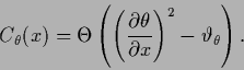
The expression  of Eq. (521)
can be generalized to
of Eq. (521)
can be generalized to
 |
(523) |
where,
analogously to Eq. (500),
![\begin{displaymath}
\omega_\theta(x)
=
\int \!dx^\prime \,
{\bf W}_\theta(x,x^\prime)
[\theta(x^\prime)-t_\theta(x^\prime)]
,
\end{displaymath}](img1819.png) |
(524) |
and
 is some filter operator acting on the hyperfield
and
is some filter operator acting on the hyperfield
and
 is a template for the hyperfield.
Discontinuous functions can either be approximated
by using discontinuous templates  or by eliminating matrix elements of the inverse covariance
which connect the two sides of the discontinuity.
For example, consider the discrete version
of a negative Laplacian
with periodic boundary conditions,
or by eliminating matrix elements of the inverse covariance
which connect the two sides of the discontinuity.
For example, consider the discrete version
of a negative Laplacian
with periodic boundary conditions,
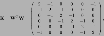 |
(525) |
and possible square root,
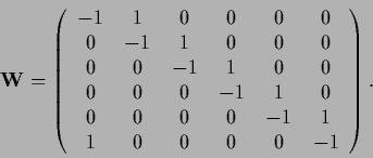 |
(526) |
The first three points
can be disconnected from the last three points
by setting
 and
and
 to zero, namely,
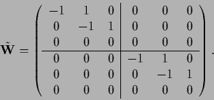 |
(527) |
so that
the smoothness prior with inverse covariance
 |
(528) |
is ineffective
between points from different regions,
In contrast to using discontinuous templates,
the height of the jump at the discontinuity
has not to be given in advance
when
using such disconnected Laplacians (or other inverse covariances).
On the other hand
training data are then required for all separated regions
to determine the free constants
which correspond to the zero modes of the Laplacian.
Non-Gaussian priors,
which will be discussed in more detail in the next Section,
often provide an alternative
to the use of function hyperparameters.
Similarly to Eq. (521)
one may for example
define a binary function  in terms of ,
 |
(529) |
like, for a negative Laplacian prior,
 |
(530) |
Here is directly determined by
and is not considered as an independent hyperfield.
Notice also that the functions  and may be nonlocal with respect to
  ,
meaning they may depend on more than one value.
The threshold has to be related to
the prior expectations on
,
meaning they may depend on more than one value.
The threshold has to be related to
the prior expectations on  .
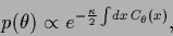
A possible non-Gaussian prior for formulated in terms of
.
A possible non-Gaussian prior for formulated in terms of  can be,
 |
(531) |
with
 counting the number of discontinuities of .
Alternatively to
counting the number of discontinuities of .
Alternatively to  one may for a real define,
similarly to (523),
one may for a real define,
similarly to (523),
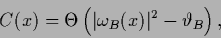 |
(532) |
with
![\begin{displaymath}
\omega_B(x)
=
\int \!dx^\prime \,
{\bf W}_B(x,x^\prime)
[B(x^\prime)-t_B(x^\prime)]
,
\end{displaymath}](img1838.png) |
(533) |
and some filter operator
 and template
 .
Similarly to the introduction of hyperparameters,
one can treat
formally as an independent function
by including a term
.
Similarly to the introduction of hyperparameters,
one can treat
formally as an independent function
by including a term
 in the prior energy
and taking the limit
in the prior energy
and taking the limit
 .
.
Eq. (531) looks similar to
the combination of the prior (504)
with the hyperprior (522),
 |
(534) |
Notice, however, that the definition (505) of
the hyperfield  (and
(and  or , respectively),
is different from that of (and or
or , respectively),
is different from that of (and or  ),
which are direct functions of .
If the differ only in their templates,
the normalization term can be skipped.
Then, identifying in (534)
with a binary and assuming
= ,
),
which are direct functions of .
If the differ only in their templates,
the normalization term can be skipped.
Then, identifying in (534)
with a binary and assuming
= ,
 =
=  ,
= ,
the two equations are equivalent
for
=
,
= ,
the two equations are equivalent
for
=
 .
In the absence of hyperpriors,
it is indeed easily seen
that this is a selfconsistent solution for ,
given .
In general, however, when
hyperpriors are included,
another solution for
may have a larger posterior.
Non-Gaussian priors will be discussed
in Section 6.5.
.
In the absence of hyperpriors,
it is indeed easily seen
that this is a selfconsistent solution for ,
given .
In general, however, when
hyperpriors are included,
another solution for
may have a larger posterior.
Non-Gaussian priors will be discussed
in Section 6.5.
Hyperpriors or non-Gaussian prior terms
are useful to enforce specific
global constraints for or .
In images, for example, discontinuities
are expected to form closed curves.
Hyperpriors, organizing discontinuities along lines or closed curves,
are thus important for image segmentation
[70,153,66,67,238,247].
Next: Non-Gaussian prior factors
Up: Parameterizing priors: Hyperparameters
Previous: Integer hyperparameters
Contents
Joerg_Lemm
2001-01-21
![$\displaystyle \int\! dx\,dx^\prime\,
[\phi(x)-t(x)]
\, {\bf K}^T(x,x^{\prime}) \,
[\phi(x^{\prime})-t(x^{\prime})]$](img1747.png)
![$\displaystyle \int\! dx\,dx^\prime\, dx^{\prime\prime}\,
[\phi(x)-t(x)]
{\bf W}^T(x,x^{\prime})$](img1748.png)