Solving learning problems numerically
by discretizing the ![]() and
and ![]() variables
allows in principle to deal with
arbitrary non-Gaussian priors.
Compared to Gaussian priors, however,
the resulting stationarity equations are intrinsically nonlinear.
variables
allows in principle to deal with
arbitrary non-Gaussian priors.
Compared to Gaussian priors, however,
the resulting stationarity equations are intrinsically nonlinear.
As a typical example let us formulate a prior
in terms of nonlinear and non-quadratic
``potential'' functions ![]() acting on ``filtered differences''
acting on ``filtered differences''
![]() =
=
![]() ,
defined with respect to some
positive (semi-)definite inverse covariance
,
defined with respect to some
positive (semi-)definite inverse covariance
![]() =
=
![]() .
In particular, consider a prior factor
of the following form
.
In particular, consider a prior factor
of the following form
For differentiable ![]() function
the functional derivative with respect to
function
the functional derivative with respect to ![]() becomes
becomes
| (596) |
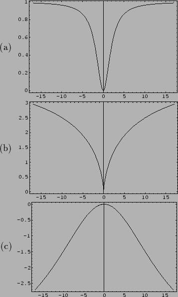
The potential functions ![]() may be fixed in advance for a given problem.
Typical choices to allow discontinuities
are symmetric ``cup'' functions
with minimum at zero and flat tails
for which one large step is cheaper than many small ones
[238]).
Examples are shown in Fig. 12 (a,b).
The cusp in (b), where the derivative does not exist,
requires special treatment [246].
Such functions can also be interpreted in the sense of robust statistics
as flat tails reduce
the sensitivity with respect to outliers
[100,101,67,26].
may be fixed in advance for a given problem.
Typical choices to allow discontinuities
are symmetric ``cup'' functions
with minimum at zero and flat tails
for which one large step is cheaper than many small ones
[238]).
Examples are shown in Fig. 12 (a,b).
The cusp in (b), where the derivative does not exist,
requires special treatment [246].
Such functions can also be interpreted in the sense of robust statistics
as flat tails reduce
the sensitivity with respect to outliers
[100,101,67,26].
Inverted ``cup'' functions, like those
shown in Fig. 12 (c),
have been obtained by optimizing a set of ![]() with respect to a sample of natural images
[246].
(For statistics of natural images
their relation to wavelet-like filters and sparse coding
see also
[175,176].)
with respect to a sample of natural images
[246].
(For statistics of natural images
their relation to wavelet-like filters and sparse coding
see also
[175,176].)
 |
While, for ![]() which are differential operators,
cup functions promote smoothness,
inverse cup functions can be used to implement
structure.
For such
which are differential operators,
cup functions promote smoothness,
inverse cup functions can be used to implement
structure.
For such ![]() the gradient algorithm for minimizing
the gradient algorithm for minimizing ![]() ,
,
| (600) |
| (601) |
Alternatively to fixing ![]() in advance
or, which is sometimes possible for low-dimensional
discrete function spaces like images,
to approximate
in advance
or, which is sometimes possible for low-dimensional
discrete function spaces like images,
to approximate ![]() by sampling from the prior distribution,
one may also introduce hyperparameters
and adapt potentials
by sampling from the prior distribution,
one may also introduce hyperparameters
and adapt potentials ![]() to the data.
to the data.
For example, attempting to adapt a unrestricted function
![]() with hyperprior
with hyperprior ![]() by
Maximum A Posteriori Approximation
one has to solve the stationarity condition
by
Maximum A Posteriori Approximation
one has to solve the stationarity condition
| (602) |
 |
(603) |
| (605) |
| (606) |
Introducing hyperparameters one has to keep in mind that the resulting additional flexibility must be balanced by the number of training data and the hyperprior to be useful in practice.