Next: General loss functions and
Up: Bayesian decision theory
Previous: Loss and risk
Contents
Loss functions for approximation
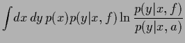
Log-loss:
A typical loss function for density estimation problems
is the log-loss
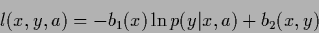 |
(46) |
with some  -independent
  ,
,  and
actions describing probability densities
and
actions describing probability densities
 |
(47) |
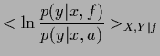
Choosing =  and
and  =
=  gives
gives
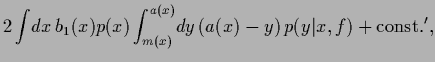
which shows that minimizing log-loss is equivalent to minimizing
the ( -averaged) Kullback-Leibler entropy
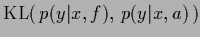 [122,123,13,46,53].
While the paper will concentrate on log-loss
we will also give a short summary of loss functions
for regression problems.
(See for example [16,201] for details.)
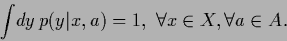
Regression problems are special density estimation problems
where the considered possible actions are restricted to
 -independent functions
  .
.
Squared-error loss:
The most common loss function for regression problems
(see Sections 3.7, 3.7.2)
is the squared-error loss. It reads
for one-dimensional
 |
(51) |
with arbitrary and .
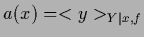
In that case the optimal function is
the regression function of the posterior
which is the mean of the predictive density
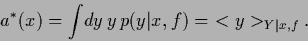 |
(52) |
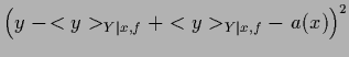
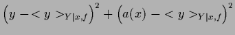
This can be easily seen by writing
where the first term in (54) is independent of
and the last term vanishes after integration over
according to the definition of  .
Hence,
.
Hence,
 |
(55) |
This is minimized by
 .
Notice that for Gaussian
.
Notice that for Gaussian  with fixed variance
log-loss and squared-error loss are equivalent.
For multi-dimensional
one-dimensional loss functions like Eq. (51)
can be used
when the component index of is considered part of the -variables.
Alternatively, loss functions depending explicitly on multidimensional
can be defined.
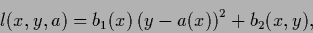
For instance, a general quadratic loss function would be
with fixed variance
log-loss and squared-error loss are equivalent.
For multi-dimensional
one-dimensional loss functions like Eq. (51)
can be used
when the component index of is considered part of the -variables.
Alternatively, loss functions depending explicitly on multidimensional
can be defined.
For instance, a general quadratic loss function would be
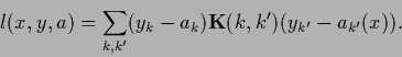 |
(56) |
with symmetric, positive definite kernel
 .
.
Absolute loss:
For absolute loss
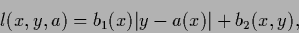 |
(57) |
with arbitrary and .
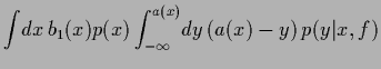
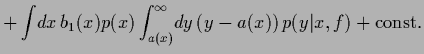
The risk becomes
where the integrals have been rewritten as
 =
=
 +
+
 and
and
 =
=
 +
+
 introducing a median function
  which satisfies
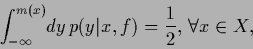 |
(60) |
so that
 |
(61) |
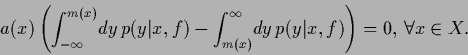
Thus the risk is minimized by any median function .
 -loss and
  - loss :
Another possible loss function,
typical for classification tasks
(see Section 3.8),
like for example image segmentation
[153],
is
the -loss for continuous
or --loss for discrete
- loss :
Another possible loss function,
typical for classification tasks
(see Section 3.8),
like for example image segmentation
[153],
is
the -loss for continuous
or --loss for discrete
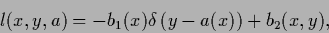 |
(62) |
with arbitrary and .
Here denotes
the Dirac -functional
for continuous
and the Kronecker for discrete .
Then,
 |
(63) |
so the optimal
corresponds to any mode function
of the predictive density.
For Gaussians mode and median are unique,
and coincide with the mean.
Next: General loss functions and
Up: Bayesian decision theory
Previous: Loss and risk
Contents
Joerg_Lemm
2001-01-21