


Next: Gaussian priors for parameters
Up: Parameterizing likelihoods: Variational methods
Previous: Parameterizing likelihoods: Variational methods
Contents
Approximate
solutions of the error minimization problem are obtained
by restricting the search (trial) space for  =
=  (or
(or  in regression).
Functions
in regression).
Functions  which are in the considered search space are
called trial functions.
Solving a minimization problem in some restricted trial space
is also called a variational approach
[97,106,29,36,27].
Clearly, minimal values obtained by
minimization within a trial space can only be larger or equal
than the true minimal value,
and from two variational approximations
that with smaller error is the better one.
which are in the considered search space are
called trial functions.
Solving a minimization problem in some restricted trial space
is also called a variational approach
[97,106,29,36,27].
Clearly, minimal values obtained by
minimization within a trial space can only be larger or equal
than the true minimal value,
and from two variational approximations
that with smaller error is the better one.
Alternatively,
using parameterized functions can also be interpreted
as implementing the a priori information
that is known to have that specific parameterized form.
(In cases where is only known
to be approximately of a specific parameterized form,
this should ideally be implemented using a prior with a parameterized template
and the parameters be treated as hyperparameters
as in Section 5.)
The following discussion holds for both interpretations.
Any parameterization =
 together with a range of allowed values
for the parameter vector
together with a range of allowed values
for the parameter vector  defines a possible trial space.
Hence we consider the error functional
defines a possible trial space.
Hence we consider the error functional
 |
(352) |
for depending on parameters
and  =
=
 .
In the special case of Gaussian regression
this reads
.
In the special case of Gaussian regression
this reads
 |
(353) |
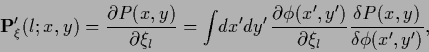
Defining the matrix
 |
(354) |
the stationarity equation for the functional (352)
becomes
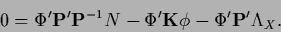 |
(355) |
Similarly,
a parameterized functional  with non-zero template
  as in (226) would give
 |
(356) |
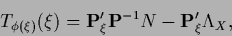
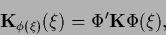
To have a convenient notation when solving for  we introduce
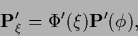 |
(357) |
i.e.,
 |
(358) |
and
 |
(359) |
to obtain for Eq. (355)
 |
(360) |
For a parameterization
restricting the space of possible  the matrix
 is not square
and cannot be inverted.
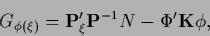
Thus, let
is not square
and cannot be inverted.
Thus, let
 be the Moore-Penrose inverse of
, i.e.,
be the Moore-Penrose inverse of
, i.e.,
 |
(361) |
and symmetric
 and
and
 .
A solution for exists
if
.
A solution for exists
if
 |
(362) |
In that case the solution can be written
 |
(363) |
with arbitrary vector  and
and
 |
(364) |
from the right null space of
,
representing a solution of
 |
(365) |
Inserting for
 Eq. (363)
into the normalization condition
=
Eq. (363)
into the normalization condition
=
 gives
gives
 |
(366) |
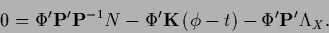
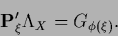
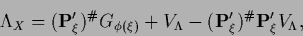
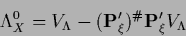
Substituting back in Eq. (355)
is eliminated yielding as stationarity equation
 |
(367) |
where  has to fulfill Eq. (362).
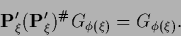
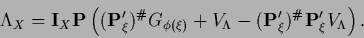
Eq. (367) may be written in a form
similar to Eq. (193)
has to fulfill Eq. (362).
Eq. (367) may be written in a form
similar to Eq. (193)
 |
(368) |
with
 |
(369) |
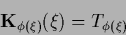
but with
 |
(370) |
being in general a nonlinear operator.
Next: Gaussian priors for parameters
Up: Parameterizing likelihoods: Variational methods
Previous: Parameterizing likelihoods: Variational methods
Contents
Joerg_Lemm
2001-01-21