


Next: Mixture models
Up: Parameterizing likelihoods: Variational methods
Previous: Gaussian priors for parameters
Contents
Solving a density estimation problem numerically,
the function  has to be discretized.
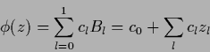
This is done by expanding in a basis
has to be discretized.
This is done by expanding in a basis
 (not necessarily orthonormal)
and,
choosing some
(not necessarily orthonormal)
and,
choosing some  ,
truncating the sum to terms with
,
truncating the sum to terms with
 ,
,
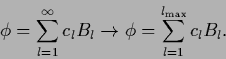 |
(380) |
This, also called Ritz's method, corresponds
to a finite linear trial space
and is equivalent
to solving a projected stationarity equation.
Using a discretization (380)
the functional (187)
becomes
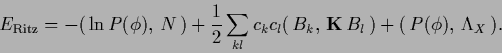 |
(381) |
Solving for the coefficients  ,
to minimize the error results
according to Eq.[355) and
,
to minimize the error results
according to Eq.[355) and
 |
(382) |
in
 |
(383) |
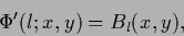
corresponding to the -dimensional equation
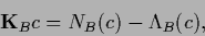 |
(384) |
with
Thus, for an orthonormal basis
Eq. (384) corresponds
to Eq. (189) projected into the trial space
by the projector
 .
.
The so called linear models are obtained by the
(very restrictive) choice
 |
(389) |
with  and
and
 = 1 and =
  .
Interactions, i.e., terms proportional to
products of
.
Interactions, i.e., terms proportional to
products of  -components like
  can be included.
Including all possible interaction would correspond to a
multidimensional Taylor expansion
of the function
can be included.
Including all possible interaction would correspond to a
multidimensional Taylor expansion
of the function  .
.
If the functions  are also parameterized
this leads to mixture models for .
(See Section 4.4.)
are also parameterized
this leads to mixture models for .
(See Section 4.4.)
Next: Mixture models
Up: Parameterizing likelihoods: Variational methods
Previous: Gaussian priors for parameters
Contents
Joerg_Lemm
2001-01-21